Google Sheets Dropdown Chips – I’m gonna love this!
Today’s helpful tip when I logged in to Google Sheets was how to use “Dropdown Chips.”
Some people I work with rely heavily on Google Sheets to share tasks like price updates. There are several repetitive fields, such as the one I label “TYPE” to tell if an item is retail, wholesale, or bulk, and if it is eligible for free shipping.
Today, I am creating a dropdown so workers can quickly select the correct “TYPE” instead of trying to remember or look up codes.
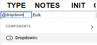
@dropdown
Typing “@dropdown” in the first cell where I want to have dropdowns opens the options you need. Under components, click “Dropdowns.”
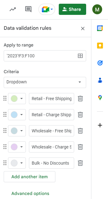
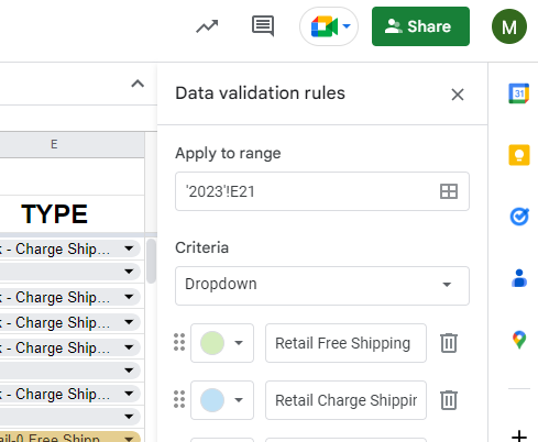
Data validation rules
Clicking Dropdowns should open a “Data validation rules” panel on the right-hand panel.
Apply to range has three sections:
Sheet Name ( ‘2023’ )
Separator ( ! )
Cell Range ( F3 )
Sheet1!K3 = Column K, Row 3 on the default Sheet1
‘2023’!K3:K100 = Column K, rows 3-100 on the sheet named 2023.
‘Price Changes’!C2:M2 = Columns C – M, Row 2 on the sheet named Price Changes.
Criteria should be left on Dropdown since we are making a dropdown.
Items can be color-coded and you can type in the text. Click the 6 dots to the left to drag and drop rearrange. Click the trash can to the right if you need to delete an option.
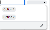
Editing Google Sheets Dropdown Chips
To edit, just click one of the dropdown cells. The bottom-right under your options should be a pencil icon. Click the pencil to open back up the Data Validation Rules panel.
Google Sheets Dropdown Menu vs Dropdown Chips
I am curious why they chose to call these Google Sheets Dropdown Chips instead of a Google Sheets Dropdown Menus. Is the name for fun? Or does it have a specific meaning?